Haven’t read Part One of this series? Click here.

The Context

You are the sole proprietor of Pearson’s Pizza, a local pizza shop. Out of nepotism and despite his weak math skills, you’ve hired your nephew Lloyd to run the joint. And because you want your business to succeed, you decide this is a good time to strengthen your stats knowledge while you teach Lloyd – after all,

“In learning you will teach, and in teaching you will learn.”

– Latin Proverb and Phil Collins

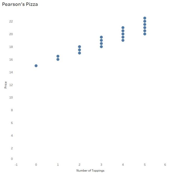
Your pizzas are priced as follows:

Cheese pizza (no toppings): $15

Additional toppings: $1/each for regular, $1.50 for premium

When we left off, you and Lloyd were exploring the relationship between the number of toppings to the pizza price using a sample of possible scenarios.

The Purpose(s) of a “Regression” Line

When investigating data sets of two continuous, numerical variables, a scatterplot is the typical go-to graph of choice. (See Daniel Zvinca’s article for more on this, and other options.)

So. When do we throw in a “line of best fit”? The answer to that question may surprise you:

A “line of best” fit, a regression line, is used to: (1) assess the relationship between two continuous variables that may respond or interact with each other (2) predict the value of y based on the value of x.

In other words, a regression line may not add value to Lloyd’s visualization if it won’t help him predict pizza prices from the number of toppings ordered. 

The equation: pizza price = 1.25*Toppings +15

Recall the slope of the line above says that for every additional topping ordered the price of the pizza will increase by $1.25.

In the last post you discussed some higher-order concepts with Lloyd, like the correlation coefficient (R) and R-Squared. Using the data above, you said, “89.3% of the variability (differences) in pizza prices can be explained by the number of toppings.” Which also means 10.7% of the variability can be explained by other variables, in this case the two types of toppings.

Since there is a high R-Squared value, does Pearson’s Pizza have a solid model for prediction purposes? Before you answer, consider the logic behind “least-squares regression.”

Least-Squares Regression

You and Lloyd now understand that “trend lines”, “lines-of-best-fit”, and “regression lines” are all different ways of saying, “prediction lines.”

The least-squares regression line, the most common type of prediction line, uses regression to minimize the sum of the squared vertical distances from each observation (each point) to the regression line. These vertical distances, called residuals, are found simply by subtracting the predicted pizza price from the actual pizza price for each observed pizza purchase.

The magnitude of each residual indicates how much you’ve over- or under- predicted the pizza price, or prediction error.

Note the green lines in the plot below:

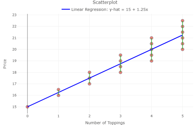
Lloyd learns about residuals

Recall, the least-squares regression equation:

pizza price = 1.25(toppings) + 15

Lloyd says he can predict the price of a pizza with 12 toppings:

pizza price =1.25*12 + 15

pizza price = $30

Sure, it’s easy to take the model and run with it. But what if the customer ordered 12 PREMIUM toppings? Logic says that’s (1.50)*12 + 15 = $33.

You explain to Lloyd that the residual here is 33 – 30, or $3. When a customer orders a pizza with 12 premium toppings, the model UNDER predicts the price of the pizza by $3. 

How valuable is THIS model for prediction purposes? Answer: It depends how much error is acceptable to your business and to your customer. 

Why the Residuals Matter

To determine if a linear model is appropriate, protocol* says to create a residual plot and check the graph of residuals. That is, graph all x-values (# of toppings) against the residuals and look for any obvious patterns. Create a residual plot with your own data here.

Ideally, the graph will show a cloud of points with no pattern. Patterns in residual plots suggest a linear model may NOT be suitable for prediction purposes.

You notice from the residual plot above, as the number of toppings increase, the residuals increase. You realize the prediction error increases as we predict for more toppings. For Pearson’s Pizza, the least-squares regression line may not be very helpful for predicting price from toppings as the number of toppings increases.

Is a residual plot necessary? Not always. The residual plot merely “zooms in” on the pattern surrounding the prediction line. Becoming more aware of residuals and the part they play in determining model fit helps you look for these patterns in the original plots. In larger data sets with more variability, however, patterns may be difficult to find.

Lloyd says, “But the p-value is significant. It’s < 0.0001. Why look at the visualization of the residual plot when the p-value is so low?”

Is Lloyd correct?! Find out in Part 3 of this series.

Summary

Today Lloyd learned a regression line has adds little to no value to his visualization if it won’t help him predict pizza prices from the number of toppings ordered.

As the owner of a prestigious pizza joint, you realize the importance of visualizing both the scatterplot and the residual plot instead of flying blind with correlation, R-Squared, and p-values alone.

Understanding residuals is one key to determining the success of your regression model. When you decide to use a regression line, keep your ultimate business goals in mind – apply the model, check the residual plot, calculate specific residuals to judge prediction error. Use context to decide how much faith to place in the magical maths.

*Full list of assumptions to be checked for the use of linear regression and how to check them here.

Want to have your own least-squares fun? This Rossman-Chance applet provides hours of entertainment for your bivariate needs. 

—Anna Foard is a Business Development Consultant at Velocity Group