Struggling with Uncertainty : The Role of Variability

“Uncertainty is the only certainty there is, and knowing how to live with insecurity is the only security.”
― John Allen Paulos

What is Uncertainty and Why Does it Matter?

At a high level, “uncertainty” is the unknown. You might believe it’s as abstract as chaos, but in fact a truth does exist – a “true” value, or parameter is out there – we just don’t know it. In fact, uncertainty is a certainty when working with data. We use samples of data in time to make decisions on the current and future state of business. And to look for truths in data, we often estimate or use probability to attempt to capture that value, or ranges of values, based on known data/observations.

I teach people how to work with, understand, and garner insights from data. What I’ve also noticed there are two kinds of clients I’ve come across in the consulting world:

Those who would like to learn HOW to visualize, measure, and understand uncertainty to help make better organizational decisions.
Those who have never considered the impact of uncertainty on organizational decisions.

As I suggested above, working with uncertainty starts with working with sample sets of data – whatever we can get our hands on. From our observed data, we can make generalizations about a phenomenon or event that may impact our organization by estimating the probability they will occur. We do this with point estimates, intervals, or broad language. For example:

Mr. X has a 40% chance of becoming the new CEO.
The proportion of revenue expected to come from our small business division this quarter is approximately 54%, with a 3% margin of error.
The Pacific Region will likely merge with the North Pacific Region next year.

Building probability models to uncover these predictions is another conversation for another day; however, it is possible to take a baby step towards understanding uncertainty and working with probabilities. In my opinion, the first step on that journey is learning more about how we interpret variation/variability in data. Why? Because accuracy and precision in measuring a probability depends on how well we’ve measured and contained the variability in the data. How we interpret probabilities depends on how we understand the difference between significance, and natural variation.

Variation

From Merriam-Webster:

Definition of variation

the act or process of varying : the state or fact of being varied
an instance of varying
the extent to which or the range in which a thing varies

Ah. Isn’t that helpful?

Google, save me!

Variation:

A change or difference in condition, amount, or level, typically with certain limits
A different or distinct form or version of something

Variability:

lack of consistency or fixed pattern; liability to vary or change.

Why Does Variation Matter?

Here’s the thing — there’s no need to study/use data when everything is identical. It’s the differences in everything around us that creates this need to use, understand, and communicate data. Our minds like patterns, but a distinction between natural and meaningful variation is not intuitive – yet it is important.

Considering how often we default to summary statistics in reporting, it’s not surprising that distinguishing between significant insights and natural variation is difficult. Not only is it foreign, the game changes depending on your industry and context.

What’s So Complicated About Variation?

Let’s set the stage to digest the concept of variation by identifying why it’s not an innate concept.

At young ages, kids are taught to look for patterns, describe patterns, predict the next value in a pattern. They are also asked, “which one of these is not like the other?”

But this type of thinking generally isn’t cultivated or expanded. Let’s look at some examples:

1) Our brains struggle with relative magnitudes of numbers.

We have a group of 2 red and 2 blue blocks. Then we start adding more blue blocks. At what point do we say there are more blue blocks? Probably when there are 3 blue, 2 red, right?

Instead, what if we started with 100 blocks? Or 1000? 501 red/499 still seems the same, right? Understanding how the size of the group modifies the response is learned – as sample/population size increases, variability ultimately decreases.

Something to ponder: When is $300 much different from $400? When is it very similar?

“For example, knowing that it takes only about eleven and a half days for a million seconds to tick away, whereas almost thirty-two years are required for a billion seconds to pass, gives one a better grasp of the relative magnitudes of these two common numbers.”
― John Allen Paulos, Innumeracy: Mathematical Illiteracy and Its Consequences

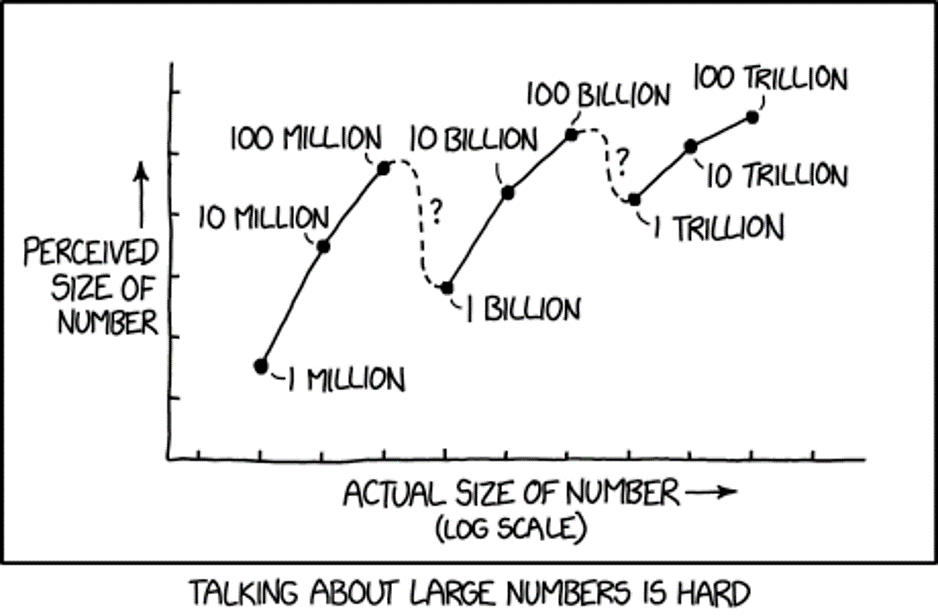
We understand that 100 times 10 is 1000. And mathematically, we understand that 1 Million times 1000 is 1 Billion. What our brains fail to recognize is the difference between 1000 and 100 is only 900, but the difference between 1 million and 1 billion is 999,000,000! We have trouble with these differences in magnitudes:

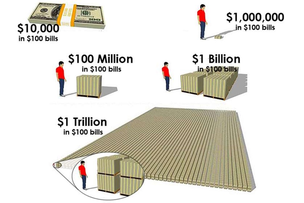
We kind of “glaze” over these concepts in U.S. math classes. But they are not intuitive!

2) We misapply the Law of Large Numbers

My favorite example misapplying the Law of Large Numbers is called The Gambler’s Fallacy, or Monte Carlo Fallacy. Here’s an easy example:

Supposed I flip a fair coin 9 times in a row and it comes up heads all 9 times, what is your prediction for the 10th coin flip? If you said tails because you think tails is more likely, you just fell for the Gambler’s Fallacy. In fact, the probability for each coin flip is exactly the same each time AND each flip is independent of another. The fact that the coin came up heads 9 times in a row is not known to the coin, or gravity for that matter. It is natural variation in play.

The Law of Large Numbers does state that as the number of coin flips increase (n>100, 1000, 10000, etc), the probability of heads gets closer and closer to 50%. However, the Law of Large numbers does NOT play out this way in the short run — and casinos cash in on this fallacy.

Oh, and if you thought the 10th coin flip would come up heads again because it had just come up heads 9 times before, you are charged with a similar fallacy, called the Hot Hand Fallacy.

3) We rely too heavily on summary statistics

Once people start learning “summary statistics”, variation is usually only brought in as a discussion as a function of range. Sadly, range only considers minimum and maximum values and ignores any other variation within the data. Learning beyond “range” as a measure of variation/spread also helps hone in on differences between mean and median and when to use each.

Standard deviation and variance also measure variation; however, the calculation relies on the mean (average) and when there is a lack of normality to the data (e.g. the data is strongly skewed), standard deviation and variance can be an inaccurate measure of the spread of the data.

In relying on summary statistics, we find ourselves looking for that one number – that ONE source of truth to describe the variation in the data. Yet, there is no ONE number that clearly describes variability – which is why you’ll see people using the 5-number summary and interquartile range. But the lack of clarity in all summary statistics makes the argument for visualizing the data.

When working with any kind of data, I always recommend visualizing the variable(s) of interest first. A simple histogram, dot plot, or box-and-whisker plot can be useful in visualizing and understanding the variation present in the data.

Start Simple: Visualize Variation

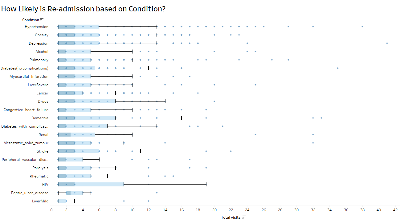
Before calculating and visualizing uncertainty with probabilities, start with visualizing variation by looking at the data one variable at a time at a granular or dis-aggregated level.

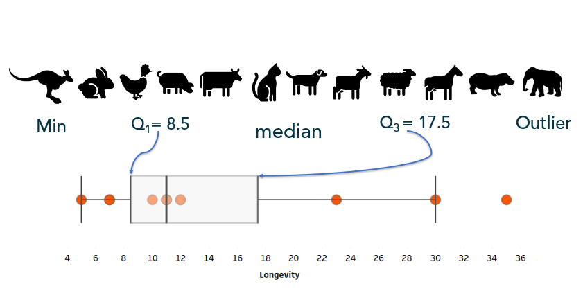
Box-and-whisker can, not only give show you outliers, these charts can also give a comparison of consistency within a variable:

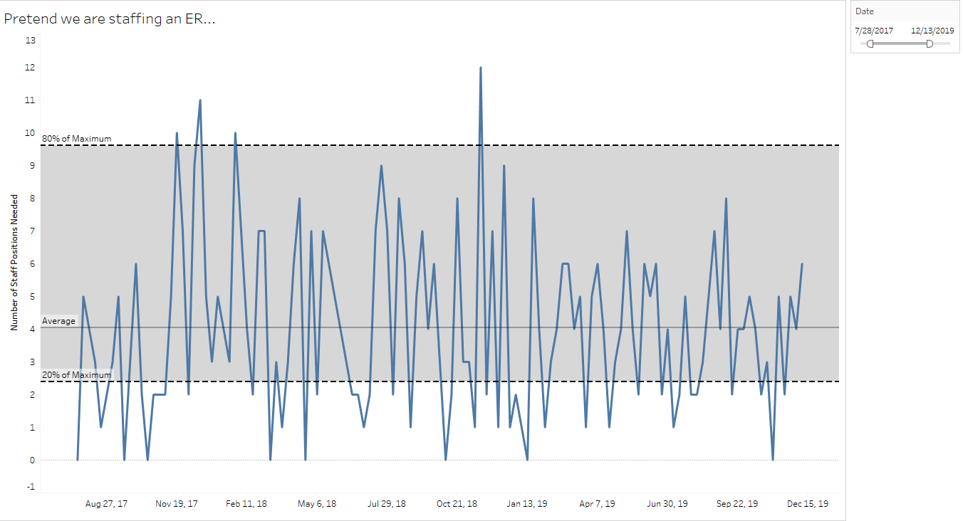
Simple control charts can capture natural variation for high-variability organizational decision-making, such as staffing an emergency room:

Think of histograms as a bar graph for continuous metrics. Histograms show the distribution of the variable (here, diameters of tortillas) over a set of bins of the same width. The width of the bar is determined by the “bin size” – smaller sets of ranges of tortilla diameters – and the height of the bar measures the frequency, or how many tortillas measured within that range. For example, the tallest bar indicates there are 26 tortillas measuring between (approximately) 6.08 and 6.10 cm.

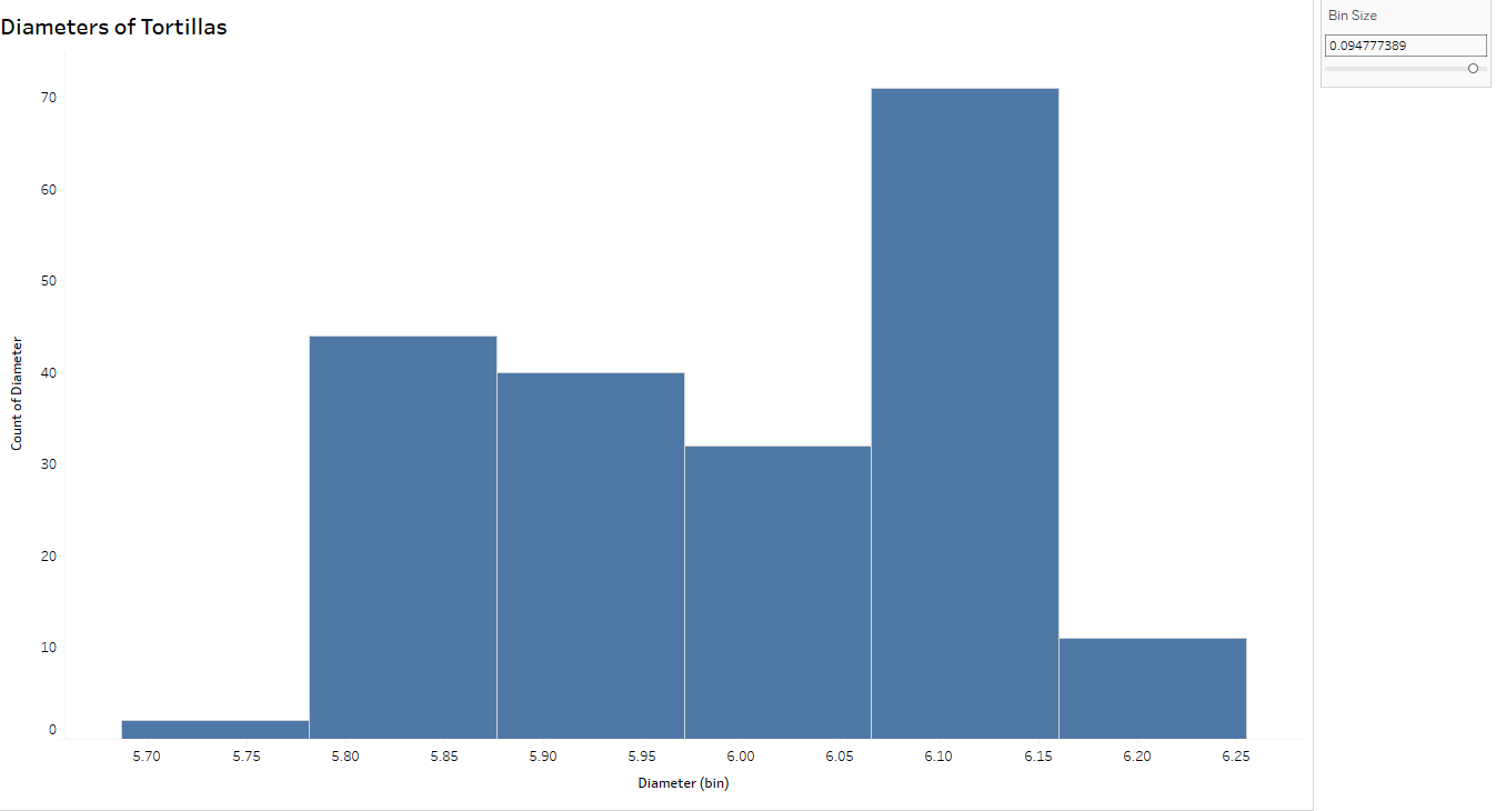
I can’t stress enough the importance of changing the bin size to explore the variation further.

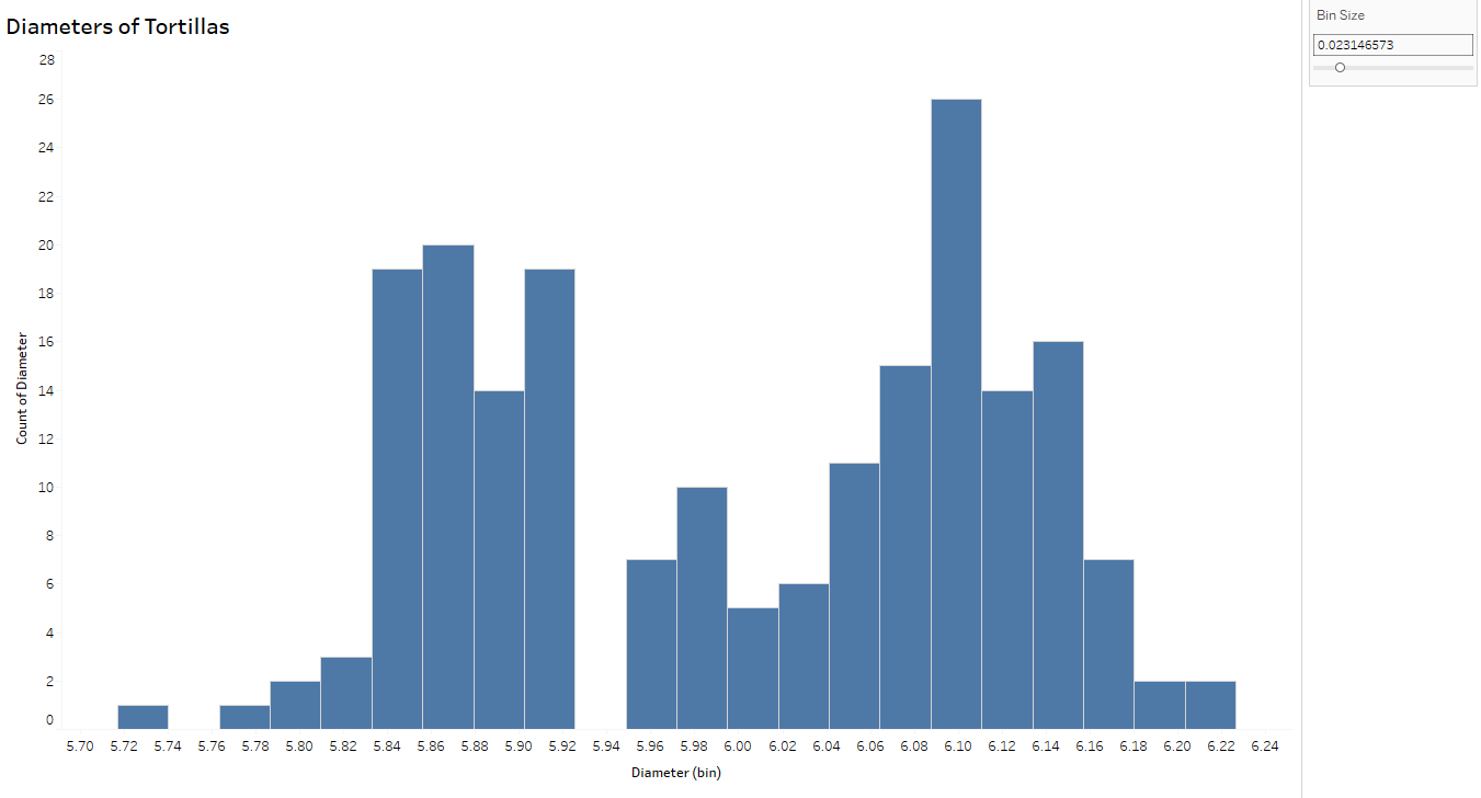
Notice the histogram with the wider bin size (below) can hide some of the variation you see above. In fact, the tortillas sampled for this process came from two separate production lines- which you can conclude from the top histogram but not below, thus emphasizing the importance of looking at variability from a more granular level.

Resources

Recently, Storytelling with Data blogged about visualizing variability. I’m also a fan of Nathan Yau’s Flowing Data post about visualizing uncertainty.

Brittany Fong has a great post about disaggregated data, as well as Steve Wexler’s post on Jitter Plots.

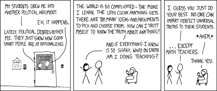
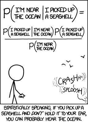
I plan a follow-up post diving more into probabilities and uncertainty. For now, I’m going to leave you with this cartoon from XKCD, called “Certainty.“

How to be the Life of the Party Part 3: Permutations and Combinations

(and why your locker combination is actually a permutation)

Welcome to the third installment of my Cheat Sheet for Stats. Be sure to check out Part 1 and Part 2.

Permutations and combinations are useful to someone interested in determining the total number of items from a set or group. This is especially helpful in probability when calculating a denominator and/or numerator.

The difference between a permutation and a combination is simple to understand – if you pay close attention to how the items/objects/people are chosen (and ignore semantics). In this post I’ll give you definitions, formulas, and examples of both permutations and combinations. But first, I’ll discuss the Fundamental Counting Principle and factorials.

The Fundamental Counting Principle

Also known as the multiplication counting rule, this principle says to multiply all possible events together to find the total number of outcomes.

A simple example starts with packing for a vacation. Say you pack 4 shirts, 3 pairs of pants, and 2 pairs of shoes. How many possible outfits can you make? (Assume they all match, or you are 5 years old and don’t give a flip.)

The fundamental counting principle says you now have:

4 * 3 * 2 = 24 possible outfits

Here’s another example. Let’s say your company requires a 5-value verification code consisting of 3 numerical values and 2 alphabetic values (in that order and case sensitive). How many possible verification codes can be produced?

Sometimes it helps to see what is going on:

And visualize the values in each position:

There are 10 total digits to consider (0 – 9) and 26 letters in the alphabet – 52 if case-sensitive. The trick is to multiply to find the total possible outcomes:

= 2,704,000 different verification codes

And what if the requirement changed to 3 numbers and 2 letters (same order), but no repeats? We’d have to take away the number of options for each digit/letter as they are used:

= 1,909,440 different verification codes

There is a little more math involved if you can put these values in any order and I won’t cover that in this post.

Factorials

At first glance, a factorial looks like a very excited number. For instance, 5! might appear to be yelling, “FIVE!” (Silly teacher joke – works better in person.) The exclamation point is actually an operator telling us to multiply that number by all integers less than that number down to 1.

Permutations

Permutations apply the Fundamental Counting Principle to determine the number of ways you can arrange members of a group. The permutation formula calculates the number of arrangements of n objects taken r at a time:

For example, let’s say you and 29 other people are in the running for 3 distinct prizes. Your names are in a hat and prizes are only given to the first, second, and third names drawn (the best prize being first). The number of ways 30 people can take first, second, and third prize is called a permutation. In a permutation, the order in which the items or people are arranged “matters”. (And by matters, you could say the order is noted, or apparent.)

don’t judge my looks, I just ran a 5K in 25:36. the first place winner didn’t show up for her prize so a nice lady held the sign so we didn’t look like chumps.

For the prize example, you can calculate this using the formula for permutations:

And this goes back to the fundamental counting principle since a portion of the numerator cancels with the denominator:

Simplifying the expression to 30*29*28 = 24,360 ways 3 individuals can be awarded first, second, and third prize from a group of 30 in a random drawing. If we were merely drawing 3 names all at once with no difference in prizes, it would NOT be considered a permutation.

Luckily you really don’t need to know the formula to calculate a permutation. The Excel function for permutations is PERMUT:

Note: There is another Excel function for permutations with repetitions – that one is PERMUTATIONA. For this example, you would use that if we drew names for the three prizes and each time the name was returned to the hat, making it possible for the same person to win all 3 times.

Combinations

Now suppose you and 29 other individuals are in the running for 3 prizes, all with the same value. Your names are in a hat and all three names are drawn at once. Because no order or arrangement is involved, this type of counting technique is called a combination. The combination formula also calculates n objects taken r at a time:

notice the denominator is different – and since you’re dividing by a larger number you can see that a combination will produce fewer possible groups than will a permutation

For the newest version of our prize example, we are taking 3 names from the hat at one time and there is no difference between prizes. Here is that calculation:

Once the 27! in the numerator and denominator cancel, we are left with the 24,360 in the numerator, but still divide by 3! (which is 3*2 = 6):

Which results in only 4060 possible combinations.

The Excel function for combinations is COMBIN:

A Locker Combination is Actually a Permutation

Combination Padlock, Not Resettable Center-Dial Location, 3/4" Shackle Height

Now consider locker combinations. Let’s assume a typical dial lock (Right, left, right) in which there are 39 numbers on the dial and your code has 3 numbers. Does order matter? Absolutely! If you try to open the lock using your 3 number code but in a different order, the locker will not open. So how many possible codes does this locker have?

If numbers couldn’t repeat, we’d have P(39,3) = 54,834 different codes (or what we call “combinations”). But if numbers could repeat, there are 39*39*39 = 59,319 possible codes – to include repeatable values, apply the PERMUTATIONA function in Excel.

You Try!

Based on what you just learned, can you spot the difference between a combination and permutation? Bonus points if you can calculate the result. (Answers at the end of the post.)

A board of directors consists of 13 people. In how many ways can a chief executive officer, a director, and a treasurer be selected?
How many ways can a jury of 12 people be selected from a group of 40 people?
A GM from a restaurant chain must select 8 restaurants from 14 for a promotional program. How many different ways can this selection be done?
At Waffle House hash browns can be ordered 18 different ways. How possible orders can be made by choosing only 3 of the 18?
A locker can have a 4-digit code. How many different codes can we have if there are 25 different numbers and numbers cannot repeat in any given code?

Answers:

Permutation. P(13,3) = 1716
Combination. C(40,12) = 5,586,853,480 order isn’t important here
Combination. C(14,8) = 3003
Combination. C(18,3) = 816
Permutation. P(25,4) = 303,600 (Repeating numbers within a code would give 390,625 different codes.)

How to Decipher False Positives (and Negatives) with Bayes’ Theorem

Note: Before proceeding, a great recap of probability concepts can be found here, written by Paul Rossman. 

But First, Conditional Probability

When I teach conditional probability, I tell my students to pay close attention to the vertical line in the formula above. Whenever they see it, they must imagine the loud baritone behind-the-scenes announcer voice from Bill Nye saying, “GIVEN!”

This symbol | always indicates we assume the event that follows it has already occurred. The formula above, then, should be read: The probability event A will occur given event B has already occurred.

A simple example of conditional probability uses the ubiquitous deck of cards. From a standard deck of 52, what is the probability you draw an ace on the second draw if you know an ace has already been drawn (and left out of the deck) on the first draw?

Since a deck of 52 playing cards contains 4 aces, the probability of drawing the first ace is 4/52. But the probability of drawing an ace given the first card drawn was an ace is 3/51 — 3 aces left in the deck with 51 total cards remaining. Hence, conditional probability assumes another event has already taken place.

False Positives and False Negatives: What They’re Not

Tests are flawed.

According to MedicineNet, a rapid strep test from your doctor or urgent care has a 2% false positive rate. This means 2% of patients who do not actually have Group A streptococcus bacteria present in their mouth test positive for the bacteria. The rapid strep test also indicates a negative result in patients who do have the bacteria 5% of the time — a false negative.

Another way to look at it: The 2% “false positive” result indicates the test displays a true positive in 98% of patients. The 5% “false negative” result means the test displays a true negative in 95% of patients.

It’s common to hear these false positive/true positive results incorrectly interpreted. These rates do not mean the patient who tests positive for a rapid strep test has a 98% likelihood of having the bacteria and a 2% likelihood of not having it. And a negative result does not indicate one still has a 5% chance of having the bacteria.

Even more confusing, but important is the idea that while a 2% false positive does indicate that 2% of patients who do not have strep test positive, it does not mean that of all positives, 2% do have strep. There is more to consider in calculating those kinds of probabilities. Specifically, we would need to know how pervasive strep is for that population in order to come close to the actual probability that someone testing positive has the bacteria.

Enter: Bayes’ Theorem

Bayes’ Theorem considers both the population’s probability of contracting the bacteria and the false positives/negatives.

I know, I know — that formula looks INSANE. So I’ll start simple and gradually build to applying the formula – soon you’ll realize it’s not too bad.

Example: Drug Testing

Many employers require prospective employees to take a drug test. A positive result on this test indicates that the prospective employee uses illegal drugs. However, not all people who test positive actually use drugs. For this example, suppose that 4% of prospective employees use drugs, the false positive rate is 5%, and the false negative rate is 10%.

Here we’ve been given 3 key pieces of information:

The prevalence of drug use among these prospective employees, which is given as a probability of 4% (or 0.04). We can use the complement rule to find the probability an employee doesn’t use drugs: 1 – 0.04 = 0.96.
The probability a prospective employee tests positive when they did not, in fact, take drugs — the false positive rate — which is 5% (or 0.05).
The probability a prospective employee tests negative when they did, in fact, take drugs — the false negative rate — which is 10% (or 0.10).

It’s helpful to step back and consider the two things are happening here: First, the prospective employee either takes drugs, or they don’t. Then, they are given a drug test and either test positive, or they don’t.

I recommend a visual guide for these types of problems. A tree diagram helps you take these two pieces of information and logically draw out the unique possibilities.

Tree diagrams are also helpful to show us where to apply the multiplication principle in probability. For example, to find the probability a prospective employee didn’t take drugs and tests positive, we multiply P(no drugs) * P(positive) = (.96)*(.05) = 0.048.

An important note: The probability of selecting a potential employee who did not take drugs and tests negative is not the same as the probability an employee tests negative GIVEN they did not take drugs. In the former, we don’t know if they took drugs or not; in the latter, we know they did not take drugs – the “given” language indicates this prior knowledge/evidence.

What’s the probability someone tests positive?

We can also use the tree diagram to calculate the probability a potential employee tests positive for drugs.

A potential employee could test positive when they took drugs OR when they didn’t take drugs. To find the probabilities separately, multiply down their respective tree diagram branches:

Using probability rules, “OR” indicates you must add something together. Since one could test positive in two different ways, just add them together after you calculate the probabilities separately:

P(positive) = 0.048 + 0.036 = 0.084

Given a positive result, what is the probability a person doesn’t take drugs?

Which brings us to Bayes’ Theorem:

Let’s find all of the pieces:

P(positive | no drugs) is merely the probability of a false positive = 0.05
P(no drugs) = 0.96
So we already calculated the numerator above when we multiplied 0.05*0.96 = 0.048
We also calculated the denominator: P(positive) = 0.084

which simplifies to

Whoa.

This means, if we know a potential employee tested positive for drug use, there is a 57.14% probability they don’t actually take drugs — which is MUCH HIGHER than the false positive rate of 0.05. In other words, if a potential employee (in this population with 4% drug use) tests positive for drug use, the probability they don’t take drugs is 57.14%

How is that different from a false positive? A false positive says, “We know this person doesn’t take drugs, but the probability they will test positive for drug use is 5%.” While if we know they tested positive, the probability they don’t take drugs is 57%.

Why is this probability so large? It doesn’t seem possible! Yet, it takes into account the likelihood a person in the population takes drugs, which is only 4%.

In math terms:

P(positive | no drugs) = 0.05 while P(no drugs | positive) = 0.5714

Which also means that if a potential employee tests positive, the probability they do indeed take drugs is lower than what you might think. You can find this probability by taking the complement of the last calculation: 1 – 0.5714 = 0.4286. OR, recalculate using the formula:

Now You Try: #DataQuiz

Back in October I posted a #DataQuiz to Twitter, with a Bayesian twist. Can you calculate the answer using this tutorial without looking at the answer (in tweet comments)?

Hints:

Draw out the situation using a tree diagram
What happens first? What happens second?
What is “given”?

Next Up: Business Applications

Stay tuned! Paul Rossman has a follow-up post that I’ll link to when it’s ready. He’s got some brilliant use case scenarios with application in Tableau.

The Monty Hall Problem

In class we discussed and debated the logic behind the ubiquitous “Monty Hall Problem“:

“Suppose you’re on a game show, and you’re given the choice of three doors: Behind one door is a car; behind the others, goats. You pick a door, say No. 1, and the host, who knows what’s behind the doors, opens another door, say No. 3, which has a goat. He then says to you, “Do you want to pick door No. 2?” Is it to your advantage to switch your choice? (Parade Magazine, Whitaker 1990)

Here is a simulation and an explanation of the answer.