As a follow-up to last week’s webinar with Andy Kriebel and Eva Murray, I’ve put together just a few common examples of means other than the ubiquitous arithmetic mean. A great deal of work on each of these topics can be found throughout the interwebs if your Googling fingers get itchy.

The Weighted Mean

My favorite of all the means. Sometimes called expected value, or the mean of a discrete random variable.

Grades

When computing a course grade or overall GPA, the weighted mean takes into account each possible outcome and how often that outcome occurs in a dataset. A weight is applied to each possible outcome — for example, each type of grade in a course — then added together to return the overall weighted mean. And since Econ was my favorite course in college…

If you have an exam average of 80, quiz/homework average of 65 and lab average of 78, what is your final grade? (Hint: Don’t forget to change percentages to decimals.)

Vegas

Weighted means are also effective for assessing risk in insurance or gambling. Also known as the expected value, it considers all possible outcomes of an event and the probability of each possible outcome. Expected values reflect a long-term average. Meaning, over the long run, you would expect to win/lose this amount. A negative expected value indicates a house advantage and a positive expected value indicates the player’s advantage (and unless you have skills in the poker room, the advantage is never on the player’s side). An expected value of $0 indicates you’ll break even in the long-run.

I’ll admit my favorite casino game is American roulette:

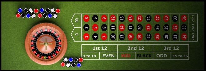
As you can see, the “inside” of the roulette table contains numbers 1-36 (18 of which are red, the other 18 black). But WAIT! Here’s how they fool you — see the numbers “0” and “00”? 0 and 00 are neither red nor black, though they do count towards the 38 total outcomes on the roulette board. When the dealer spins the wheel, a ball bounces around and chooses from numbers 1 thru 36, 0 AND 00 — that’s 38 possible outcomes.

Let’s say you wager $1 on “black”. And if the winning number is, in fact, black, you get your original dollar AND win another (putting you “up” $1). Unsuspecting victims new to the roulette table think they have a 50/50 shot at black; however, the probability of “black” is actually 18/38 and the probability of “not black” is 20/38″.

Here’s how it breaks down for you:

Just as in the grading example, each outcome (dollars made or lost) is first multiplied by its weight, where the weight here is the theoretical probability assigned to that outcome. After multiplying, add each product (outcome times probability) together. Note: Don’t divide at the end like you’d do for the arithmetic mean – it’s a common mistake, but easy to remedy if you check your work.

Some Gambling Advice: The belief that casino games adhere to some “law of averages” in the short run is called the Gambler’s Fallacy. Just because the ball on the roulette wheel landed on 5 red numbers in a row doesn’t mean it’s time for a black number on the next spin! I watched a guy lose $300 on three spins of the wheel because, as he exclaimed, “Every number has been red It’s black’s turn! It’s the law of averages!”

The Geometric Mean

A Geometric mean is useful when you’re looking to average a factor (multiplier) applied over time – like investment growth or compound interest.

I enjoyed my finance classes in school, especially the part about how compound interest works. If you think about compound interest over time, you may recall the growth is exponential, not linear. And exponential growth indicates that in order to grow from one value to the next, a constant was multiplied (not added).

As a basic example, let’s say you invest $100,000 at the beginning of 4 years. For simplicity, let’s say the growth rate followed the pattern +40%, -40%, +40%, -40% over the 4 years. At the end of 4 years, you’ve got $70,560 left.

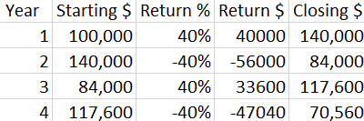
So you know your 4-year return on the investment is: (70,560 – 100,000)/100,000 = -.2944 or -29.44%. But if you averaged out the 4 growth rates using the arithmetic mean, you’d have 0%. Which is why the arithmetic mean doesn’t make sense here.

Instead, apply the geometric mean:

The Harmonic Mean

You drive 60 mph to grandma’s house and 40 mph on the return trip. What was your average speed?

Let’s dust off that formula from physics class: speed = distance/time

Since the speed you drive plays into the time it takes to cover a certain distance, that formula may clue you in as to why you can’t just take an arithmetic mean of the two speeds. So before I introduce the formula for harmonic mean, I’ll combine those two trips using the formula for speed to determine the average speed.

The set-up Distance doesn’t matter here so we’ll use 1 mile. Feel free to use a different distance to verify, but you’d be reducing fractions a good bit along the way and I’m all about efficiency. Use a distance of 1 mile for each leg of the journey and the two speeds of 40mph and 60 mph.

First determine the time it takes to go 1 mile by reworking the speed formula:

To determine the average speed, we’ll combine the two legs of the trip using the speed formula (which will return the overall, or average, speed of the entire trip):

The formula for the harmonic mean looks like this:

Where n is the number of 1-mile trips, in this example, and the rates are 40 and 60 mph:

If you scroll up and check out that last step using the speed formula (above), you’ll see the harmonic mean formula was merely a clean shortcut.

If you want more information about measures of center, check out the previous blog post — Mean, Median, and Mode: How Visualizations Help Measure What’s Typical

If your organization is looking to expand its data strategy, fix its data architecture, implement data visualization, and/or optimize using machine learning, check out Velocity Group.